Openwind has the capability to run energy captures based on a time series of wind measurements rather than a binned tabular data file. This has several benefits:
•Production of “12x24” tables of energy capture by month and hour
•Simulation of time-varying plant behaviour for ramp and load-matching studies
•Ability to estimate plant revenues given time series price data
•Assessment of effects of scheduled curtailments, e.g., for bats, noise, or shadow flicker
•Estimation of high/low temperature shutdown losses including hysteresis
•Assessment of effects of different day-time/night-time wind regimes as well as seasonal effects
•Potentially more accurate estimate of energy production due to time-varying behaviour of wakes, turbulence, air density and other parameters
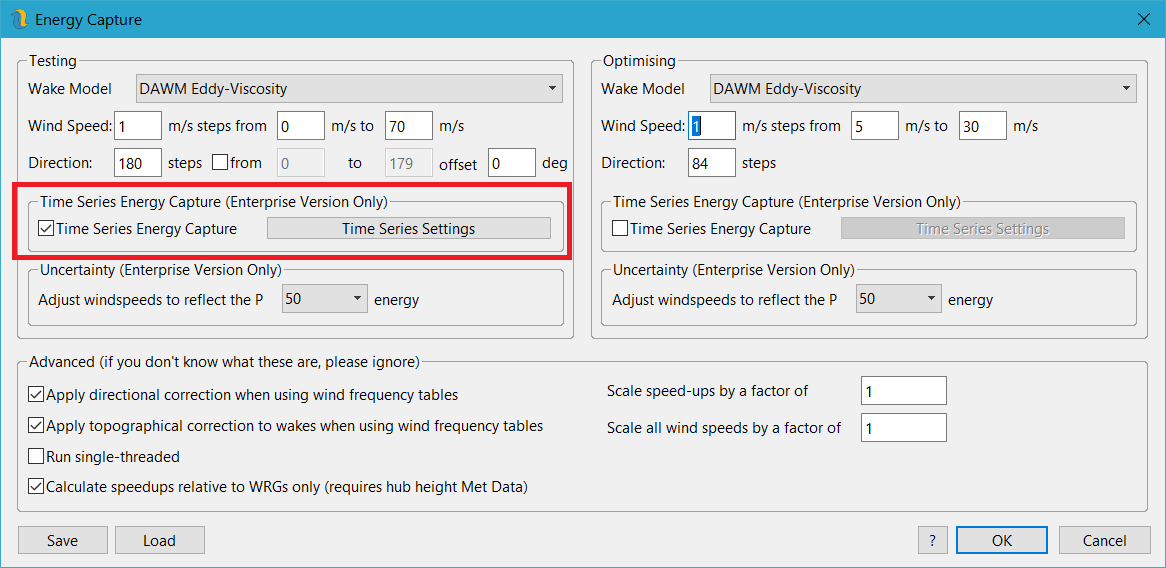
In order to use time series energy capture, it must be enabled in the energy capture options (figure 118).
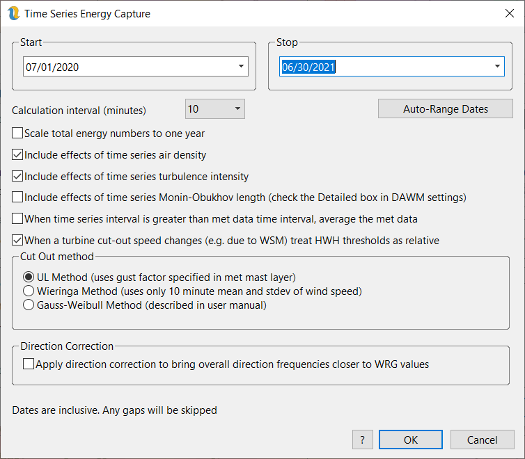
The Time Series Settings button brings up the dialog shown in figure 119. In order to run time series energy capture, the date range chosen in the Time Series Energy Capture dialog needs to be present in any met masts which will be used in the energy capture. The date range specified above in figure 119 is inclusive of the start and end days. In this case, the range starts from midnight on the morning of the July 4, 2007, to midnight on the evening of February 28, 2014.
Within this dialog are the following settings:
Calculation interval - While the interval can be anything between 1 to 60 minutes, it is recommended that the user use 1, 5, 10 or 60 minutes, depending on the mast data interval. In general, the two should be the same. If the calculation interval is larger than the recording interval of the mast data, then the data are averaged over the interval. If the interval is smaller than the data will get repeated but this is a waste of processing time and is not recommended.
•Scale total energy numbers to one year - This option scales the total energy output to one year in strict proportion to the number of missing hours in the data record. It applies no correction for seasonal variations. For example, if the mast data files contain 8000 hourly records and the number of hours in a year has been set to 8766, the total energy is increased by a factor 8766/8000.
•Include effects of time series air density - check this option to use the air density values from the time series mast data (adjusted to the turbine altitude with a constant lapse rate). Without this option, the air density at each turbine is constant throughout the energy capture.
•Include effects of time series turbulence intensity - check this option to use the turbulence intensity values from the time series mast data. With this option checked, the turbulence intensity values in the time series are scaled to the turbine location using the inverse of the WRG speed-up.
•Include effects of time series Monin-Obukhov length – this functionality is still very much in alpha mode and is intended just now to be for experimentation only.
•When time series interval is greater than met data time interval, average the met data - with this option checked, all met data variables are averaged for each TSEC time-step. When this is not checked, the first valid met data time step is used to represent the met data for the longer TSEC time-step.
•When a turbine cut-out speed changes, treat HWH thresholds as relative - This translates the high wind cut out/in behaviour to the current cut out wind speed so for example, if the normal cut out wind speed is 25m/s and we have HWH settings of 600 second 25m/s cut out, a 30 second 28m/s cut out and a 300 second 22m/s cut in and then through application of wind sector management, the cut out wind speed is changed to 15m/s, the HWH behaviour will then be translated to 600 second 15m/s cut out, a 30 second 18m/s cut out and a 300 second 12m/s cut in.
•Cut Out Method
oUL Method - the UL gust factor method uses the met mast gust factor to estimate the maximum and minimum wind speeds over different time intervals for each time step. In this method the gust factor is estimated for the met mast and then remains constant for all time steps. The met mast gust factor can be calculated externally or within Openwind using either the Gauss-Weibull or Wieringa methods.
oWieringa method - the Wieringa gust factor method uses the standard deviation of the wind speed for each time step to give a different gust factor for each time step based on the turbulence intensity. That gust factor is then used to estimate the maximum and minimum wind speeds over different time intervals for that time step.
oGauss-Weibull Method - the Gauss-Weibull method uses the turbulence intensity at each time step to estimate the gust factor for each time step based on the turbulence intensity. That gust factor is then used to estimate the maximum and minimum wind speeds over different time intervals for that time step.
•Apply direction correction to bring overall direction frequencies (and mean wind speeds) closer to WRG values - this option activates a method which creates a cumulative probability distribution from both the met mast direction field and the WRG direction probabilities at the turbine location. Then, for each time step, the direction at the met mast is used look up the corresponding cumulative probability of that direction value. This method matches the mean wind speed and direction distribution at the turbine to the values in the WRG. There is evidence (to be presented in an upcoming paper which will be linked here) that this method makes the ramp rate behaviour more realistic at the turbines.
•Auto-Range Dates – this button looks at the met masts in the workbook and attempts to come up with the longest period that is common to all masts. The method only looks at met masts which have turbines associated with them.
It is important to note that the time series energy capture is completely independent of the standard energy capture using tabular data. However, by unchecking all three options (time series air density; time series turbulence intensity; time series turbulence intensity), the time series energy capture should reproduce the results of the standard energy capture very closely, so long as the frequency table is derived from the same time series data.
The capability to run time series energy capture introduces important considerations regarding the meteorological data. For time series energy capture calculations involving multiple masts, each time step requires valid data at every mast; wherever there are data gaps at one mast, that same record in other masts will be deemed invalid. Where some or all met masts contain significant data gaps and different met masts have different invalid periods, this can result in a significant difference in the data used for the frequency table compared to the data used for the time series energy capture. In general, it is a good idea to either fill gaps in each mast’s record, or ensure that all met masts contain the same invalid periods.
There is an important distinction between the type of time series energy capture described here and what is described in other software packages in which a probabilistic energy capture is first carried out and then a met mast time series is used to index into the table of results by wind speed and direction to produce an 8760 or 12x24. The method described here genuinely incorporates time-varying data, and therefore simulates the energy capture from first principles without reference to the probabilistic method. That is why it is easy to use this method to estimate temperature shutdown losses, or to evaluate interactive phenomena, such as interrelated effects of temperature, turbulence, wake persistence, air density, and wind speed.
Having said that, there are similarities between our time series method and the probabilistic energy capture. For example, one wind speed and direction at a time is used for the wake calculation, and the WRG is used to scale the mast wind speed before it is input to the power curve function.
The fundamental model assumptions in the time series energy capture are similar to the standard probabilistic energy capture in that the speed and direction frequency distribution at the mast takes precedence, and the WRG is used to merely scale the measured data. The constant wind speed and direction assumed in the wake model is an approximation, but it is likely to produce small errors given that the most significant wake effects are from nearby turbines, which are also likely to experience similar wind speeds and directions.
The time series energy capture also models individual turbine performance more realistically by allowing the energy generated by the turbine to vary with velocity, air density and turbulence intensity for each time step. Inflow angles are modelled separately (see Energy Losses ).
Looking towards future development, addressing the effects of phenomena such as thermal stability will require the use of a true time series energy capture such as that described here. This prospect exposes limitations in the WRG itself, which is traditionally a static file representing average relationships over all time intervals. A time-varying WRG could be useful for driving different wake model modes as well as allowing there to be different speed-up ratios at different times of day or times of year. See the section on Multi-Dimensional Wind Resource Grids for more information on creating and using time-varying WRGs.
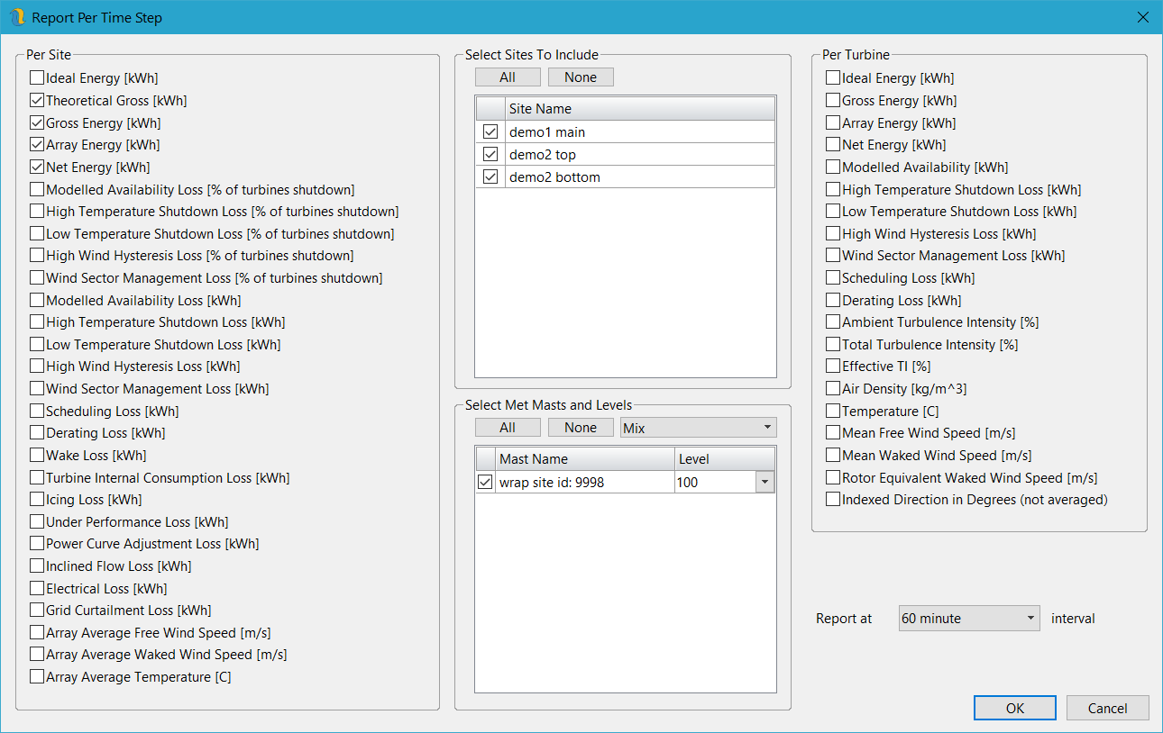
The outputs of the time series energy capture are the same as for the standard energy capture. In addition, the model produces a 12x24 matrix of energy production by hour and month for each site layer, and there is the option to output a time series with user-selected fields as shown in 120 below.
For sites with many turbines, it is expected that users will elect to output results for the entire project, whereas for small projects of a few turbines, it may be desirable to see results for each turbine.
Figure 120 shows the options available for time-series output. The panel on the right allows the user to choose for which site layers the time-series results are to be output (all site layers are included in the main body of the report but time-series output can consume a lot of space). The left-hand panel allows the user to choose which fields are output per turbine or per site layer.
The shutdown losses are reported for the modelled turbine losses only and do not include any percentage losses input through the energy loss interface but rather those modelled losses that are a part of the turbine type definition.
Please note that as energy capture results are not saved in the workbook, use of the Undo functionality will reset the energy capture results.


