Met-Mast-Layer

Users may load wind frequency tables or time series data into Openwind as MetMastLayers. A MetMastLayer represents the wind speed and direction measurements taken at a single meteorological measuring mast at a single measurement height. The user is assumed to have carried out any long-term adjustment and quality control necessary to convert the original time series into a usable data set and the resulting data has then been binned by wind speed and direction into a wind frequency table.

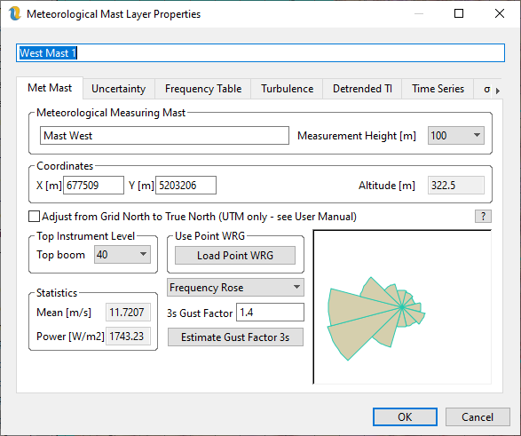
Figure 1: MetMastLayer Properties: Met Mast Tab

The data describing the main properties of the met mast are displayed in the Met Mast tab shown in figure 1.

If the MetMastLayer has access to terrain data (via the layer hierarchy), the altitude box will show the altitude of the base of the mast. The measurement height is the height above ground level at which the wind speed and direction were measured.

The gust factor is used when estimating the high wind hysteresis loss. The IEC default is 1.4 but this can be a little bit conservative. Openwind does not have access to the data required to calculate the gust factor but it is not unreasonable to think that it may be related to the 99.5th percentile of the standard deviation and this is the value that is calculated from the time-series tab when the Estimate Gust Factor button is pressed.

Uncertainty

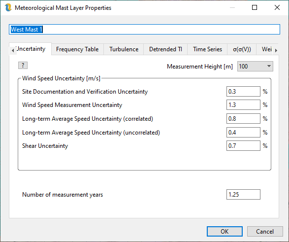
Figure 2: MetMastLayer Properties: Uncertainty Tab

The uncertainty tab should contain estimates of the various sources of uncertainty in the met mast wind speed data. These estimates can be exported as part of the met mast CSV file (e.g. by Windographer) and can vary by height. If you have a multi-height met mast then it is likely that one or more, if not all, of the following will vary by height.

• Site Documentation and Verification Uncertainty - If a met mast has been audited and a site visit carried out to verify that the installation matches the documentation and that the met mast has been installed correctly, this can be set to 0%.

• Wind Speed Measurement Uncertainty – this is a function of the instrument and its calibration report, if one exists.

• Long-term Average Speed Uncertainty (correlated) – this is the uncertainty introduced by the long-term adjustment. In this case we are assuming that one mast acts as a primary and that the other masts are then adjusted to the long term using that primary mast. In that case the initial long-term adjustment of the primary mast introduces a source of uncertainty which is common to all the masts in the project.

• Long-term Average Speed Uncertainty (uncorrelated) – this is the uncertainty introduced by the long-term adjustment of a secondary mast to the primary mast. The primary mast has 0% for this category.

• Shear uncertainty – this is the uncertainty introduced by shearing above the top measurement height of the met mast up to hub height (s). If the current height is not sheared then this can be set to 0%.

• Number of measurement years – this is the only uncertainty input on this tab which does not vary by height. It can be a fraction (as shown above) and should reflect the number of years of measurements at this mast and not necessarily the length of record that has been imported.

Please see section 40 for a fuller description of how these inputs are used.

Openwind currently accepts the Risoe TAB file format as well as a simple time series comma separated text file format in table 1 and table 2.

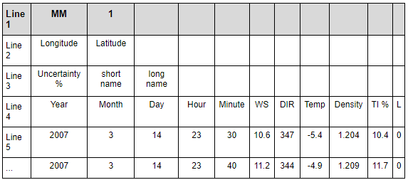
Table 1: Single Height Met Mast CSV Format

Time-Series

Windographer and UL both support output to this CSV format. The advantage of importing a time series instead of a TAB file is that we get the turbulence, temperature and density data. Openwind will bin the data into the frequency table, turbulence table and standard deviation of the standard deviation of the wind speed (used in effective TI calculations). The advantage of bringing in time series data is that we can rebin the data within Openwind as well as use the met data in time series energy captures. The MM1 format is being slowly phased out in favour of MM2.X formats (below).

Note: Some modelling applications (e.g., WAsP by Risoe) output WRGs consisting of factors describing Weibull curves. These Weibull factors may be chosen for a variety of reasons and some applications output Weibull curves whose “goodness of fit” has been valued above accurately matching the mean wind speed of the modelled distribution. For this type of data, it is necessary to load a similarly fitted point WRG to cancel out the bias introduced by the Weibull fitting procedure. When this is not the case (e.g., when using UL WRGs), then a point WRG is unnecessary. The purpose of the point WRG is to represent the equivalent of the TAB file data, only in Weibull curves. If it is not known whether the fitting procedure was set up to match the mean wind speeds, then it is safer to use a point WRG.

In the case where you do not have density data, Openwind can calculate the air density from the temperature field.

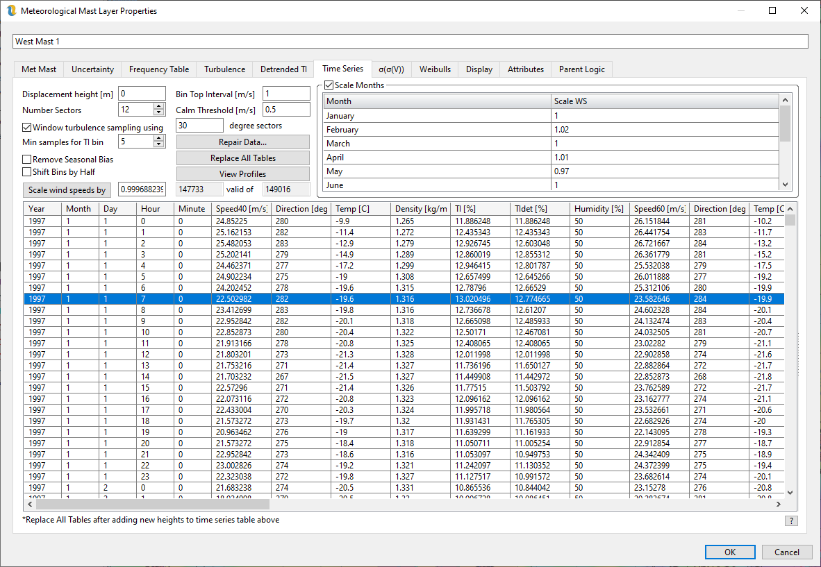
Figure 3: Met Mast Layer Time Series Tab

• Replace All Tables - populates the frequency table, the turbulence table and the Eff. TI table from the time series data using the bining rules specified above.

• Scale Months - this check box enables or disables the ability to scale the wind speeds in each month by a different user-input factor. The corresponding turbulence intensity values are scaled by the inverse of these factors. In order for these scalings to take effect, the user needs to press the Replace All Tables button.

• Scale wind speeds by - this scales all wind speeds by the factor to the right of this button. The corresponding turbulence intensity values are scaled by the inverse of this factor. Again, one should press the Replace All Tables button for this scale factor to take effect. Pressing the button causes Openwind to calculate an overall wind speed scale factor which, when combined with the monthly scale factors, maintains the original overall wind speed and automatically populates the overall wind speed scale factor with that value.

• Shift bins by half – when used with integer bins, this option sets the bin top to be on the half m/s and the bin center to be on the integer whereas by default, Openwind uses integer bin tops.

• Remove Seasonal Bias – this option weights each time step by the inverse of the number of valid records at that time-step within a notional year. If there are two years of data but with gaps then the records for time steps that are present in one year but not the other, will be weighted twice as much as records for timesteps which are valid in both years. It does nothing more sophisticated than this.

• Repair Data… - brings up the repair data dialog shown in fi57

Repair Met Data

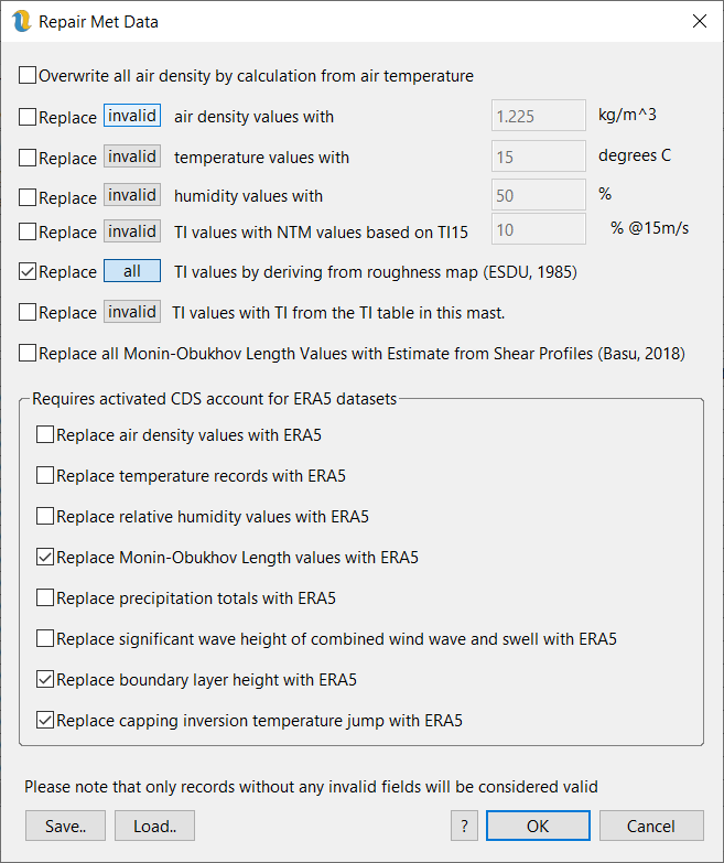
Figure 4: Repair Met Data

• Overwrite all air density by calculation from air temperature - does what it says. It is important to make sure that the met mast layer has access to terrain elevation data before running this.

• Replace invalid/all temperature records with the following value - uses the value specified in the Air temperature field.

• Replace invalid/all air density records with the following value - uses the value specified in the Air density field.

• Replace invalid/all TI records with NTM values based on TI 15 below – creates Normal Turbulence Model curves that pass through the specified value in the Turbulence Intensity field at 15 m/s.

• Replace missing invalid/all TI records by deriving from roughness map (ESDU, 1985) – taken from (Burton, Sharpe, Jenkins, & Bossanyi, 2001) pages 19-21. We calculate the mean standard deviation of the wind speed, sigma, as 2.45u* (Burton et al. say 2.5u* and Mann says 2.4u* so we split the difference). For simplicity and as a reasonable approximation we calculate the friction velocity, u*, according to where is the mean wind speed, K is the von Karman constant (~0.4) z is the instrument height, z0 is the upwind roughness and is relatively small and so can be ignored when assuming stable conditions.

• Replace missing invalid/all TI records with TI from the TI table in this mast – assuming that at least some of the records in this met mast object are valid, we can use the TI table to recreate the missing records on the basis of wind speed and direction.

• Replace all Monin-Obukhov Length Values with Estimate from Shear Profiles (Basu, 2018) - attempts to deduce MOL from the shear profiles. Only works for multi-height met data and is not great at calculating stable Monin-Obukhov lengths.

The remaining options require an account at CDS and to have downloaded data with that account from both https://cds-beta.climate.copernicus.eu/datasets/reanalysis-era5-single-levels?tab=overview and https://cds-beta.climate.copernicus.eu/datasets/reanalysis-era5-pressure-levels?tab=overview

The ERA5 UID and token need to be input into Preferences

• Replace air density values with ERA5 - uses single level hourly data for surface pressure combined with temperature in Kelvin at 2m above surface level together with the air density lapse rate specified in the workbook settings

• Replace temperature records with ERA5 - uses single level hourly data for temperature in Celsius at 2m above surface level together with the temperature lapse rate from the workbook settings.

• Replace relative humidity values with ERA5 - uses single level hourly data for temperature in Celsius at 2m above surface level together with the dewpoint temperature in Celsius at 2m above surface level.

• Replace Monin-Obukhov Length values with ERA5 - uses the formula recommended by ECMWF and draws on the single level hourly data for heat flux, dewpoint temperature in Kelvin at 2m above surface level, surface pressure, friction velocity and moisture flux.

• Replace precipitation totals with ERA5 - uses single level hourly data for total precipitation.

• Replace significant wave height of combined wind wave and swell with ERA5 - uses single level hourly data for significant height of combined wind wave and swell.

• Replace boundary layer height with ERA5 - uses single level hourly data for boundary layer height.

• Replace capping inversion temperature jump with ERA5 - uses pressure level hourly data for temperature and geopotential height. Levels are sampled down to 700hPa and then interpolated for each hour to find the temperature jump corresponding to the ABL height. It is a good idea to download the ABL height before or at the same time as this field. Please note that due to the number of levels required, this field can take many hours to download.

For all the ERA5 data there is the danger of the downloads timing out or that adjacent met masts may need to download the same data. For this reason, Openwind caches the downloaded data locally so that any repeated attempts at downloading the same data do not put additional load on the CDS servers and so that interrupted downloads can recommence where they left off.

Missing data are given the value -999. Openwind automatically parses the data using time stamps and inserts -999 data values for any missing time steps.

Each record is for the period starting at the time stamp in that record.

Frequency Table

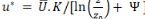
The Frequency Table tab shown in figure 5 contains the wind frequency table as it was input from the TAB file but with the numbers scaled to reflect absolute probabilities. The frequency table can also be populated from the time-series tab using Replace All Tables.

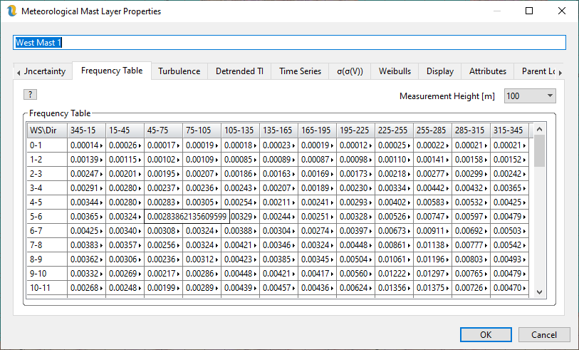
Figure 5: MetMastLayer Properties: Frequency Table Tab

In order to use wind frequency tables in energy capture calculations, each WRG needs to be able to find the appropriate MetMastLayer within its layer hierarchy. Only one MetMastLayer can be used in conjunction with each WRGLayer.

Turbulence Table

Figure 6 shows the Turbulence tab. Turbulence intensity (TI) can be input as a global value, by wind speed or by direction but the best method by far is to specify TI by wind speed and direction as shown here. This is because ambient TI drops off rapidly with increasing wind speed and is dependent on upwind roughness. Ambient TI is used to influence how the Eddy-Viscosity model behaves so it can affect the final wake loss and energy capture numbers. It is also a factor in determining turbine suitability and turbine loading. The ambient TI that a user inputs for their met mast should be calculated with as much care as the wind frequency table itself.

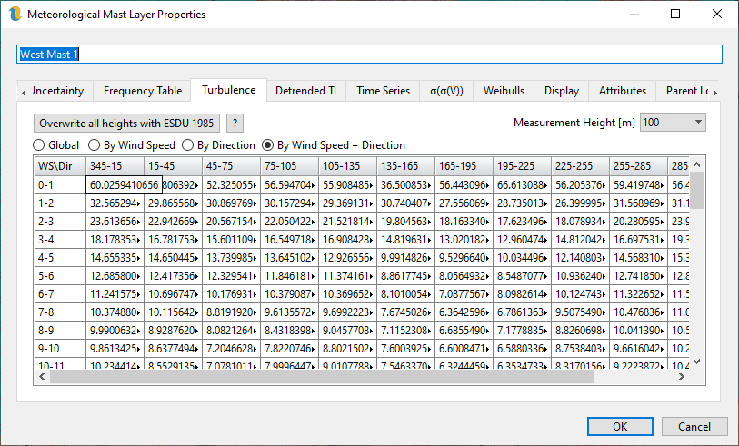
Figure 6: MetMastLayer Properties: Turbulence Tab

Detrended Turbulence Table

From v4545 onwards, we now have two turbulence tabs in Openwind. This is because IEC61400-1 recommends that any trends in the mean wind speed are removed before calculating the standard deviation of the wind speed which is then used for assessing the likely impacts of fatigue loading. However, such a recommendation does not apply to power curve testing or wake modelling and so, at least for now, it has been deemed necessary to have two versions of the turbulence intensity: one for the purposes of estimating energy yield and wake effects; and one for use when assessing loads and suitability. More information on TI detrending is given here. If TI detrended is not enabled in the workbook settings, the values in the detrended TI table will be the same as those in the regular turbulence table. Changing the setting in the workbook settings will force Openwind to detrend all detrended TI values in the workbook.

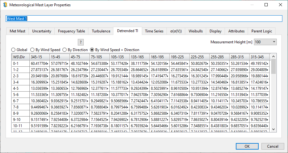
Figure 7: Detrended TI Tab

The figure above shows the detrended TI for the same met data as in the turbulence table above that.

Sigma Sigma

Figure 8 shows the σ(σ(V)) tab. The effective turbulence intensity calculation requires access to the standard deviation of the standard deviation of the wind speed. This table can also be calculated from the time series data or copied and pasted from Excel. Openwind calculates these values from the detrended TI because these values are only used in suitability and loads calculations.

Assuming that the desired approach is to use the time-series data as the basis for sigma(sigma(V)), the question inevitably arises as to what value to use in bins where there are few or no counts. To address this, Openwind fits a log curve to the data points we choose to use and then uses that log curve to fill in those bins we choose to discard.

Wind speed intervals are displayed in the first column, the raw calculated values of sigma(sigma(V)) are displayed in the second column along with the counts in the last column. The fourth column displays the data which will actually be used to calculate effective TI. Raw values are either used or discarded based on the presence or absence of a check in the third column for that row. All values used to fit the log curve are automatically used in the final output. Unused values are replaced by values from the fitted log curve.

For counts below 1000, Openwind is able to make an estimate of the uncertainty in sigma(sigma(V)). This can be used for reference when deciding which values to use.

NB: For workbooks older than v2800, it will be necessary to replace all tables in order to update the counts column to the proper values.

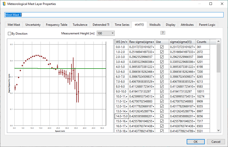
Figure 8: Standard Deviation of the Standard Deviation of Wind Speed

With the increasing use of turbulence extrapolation in Openwind, it now makes sense to offer the ability to calculate sigma(sigma(V)) by direction as well as wind speed. As shown in the table below.

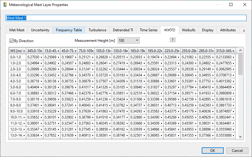
Figure 9: Sigma(Sigma(V)) by Direction and Wind Speed

The multi-height met mast format, shown in table 2, can be used to load met data at multiple heights into Openwind. This format is similar to the single height format except that it specifies a number of heights along with uncertainties (sigma) at each height. The time series data fields wind speed, direction, temperature, density, and TI are repeated for each height.

The selected height affects the data displayed in the met mast properties, the displayed wind rose and is the data level used to initialise WindMap runs.

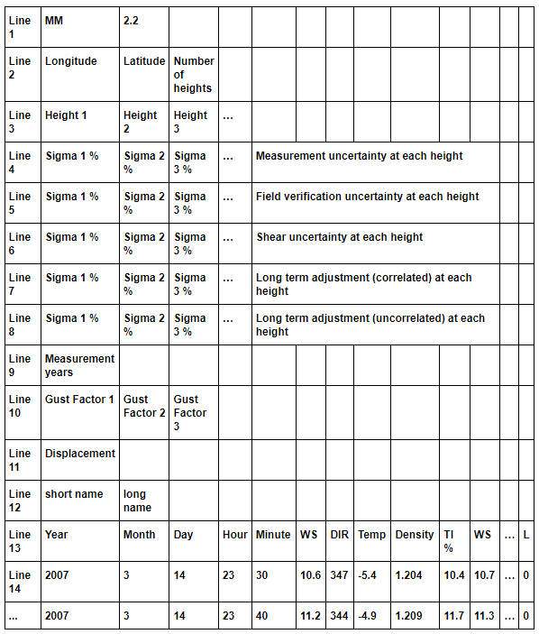
Table 2: Multi-Height Met Mast CSV Format

The Time Series tab is used to display data for all heights at once and right-clicking in the grid brings up a menu with the following options:

• Copy All - copies all the data in the grid onto the clipboard from where it can be pasted into a spreadsheet

• Copy Level - copies the data stamp columns and time series data from the mouse-clicked level to the clipboard

• Clear Data - truncates the time series to 100 records and zeros all the met data

• Remove Level - removes the level mouse-clicked

• Change Level - changes the height of the level mouse-clicked

• Add Level - adds an extra met height to the time series using one of the methods described below

• Paste - pastes data from the clipboard starting at the selected cell

MM3.2 is the latest met mast format and it is the same as MM2.2 except it starts with MM3.2 instead of MM2.2 and it has the following additional fields:

• After the TI field, for each height, add a field for relative humidity in percent

• After the Monin-Obukhov length add a field for total precipitation (rain, snow, hail, graupel etc.) in millimetres (mm) since last time-stamp.

When adding heights, Openwind can:

• Fill with -999 - probably the least useful option unless you simply want to paste data from a spreadsheet say

• Shear using roughness (takes level above if available) - uses a roughness layer to calculate shear profiles and thus the 10-minute wind speed data

• Shear between/extrapolate from adjacent heights - this is the recommended method to shear extra heights from met mast data containing two or more heights

• Shear using specified shear exponent - this is primarily for testing as it tends to add little or no useful information

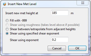
Figure 10: Options for Creating a New Met Level

Weibulls

Whilst the emphasis in Openwind moves more and more towards time-series data and time-series energy capture, it is important, for now at least, to maintain backwards compatibility with established methods. For this reason, the Weibull parameters reported in the met mast properties are based on the frequency table rather than the time-series. The differences should usually be small, but users should expect some difference.

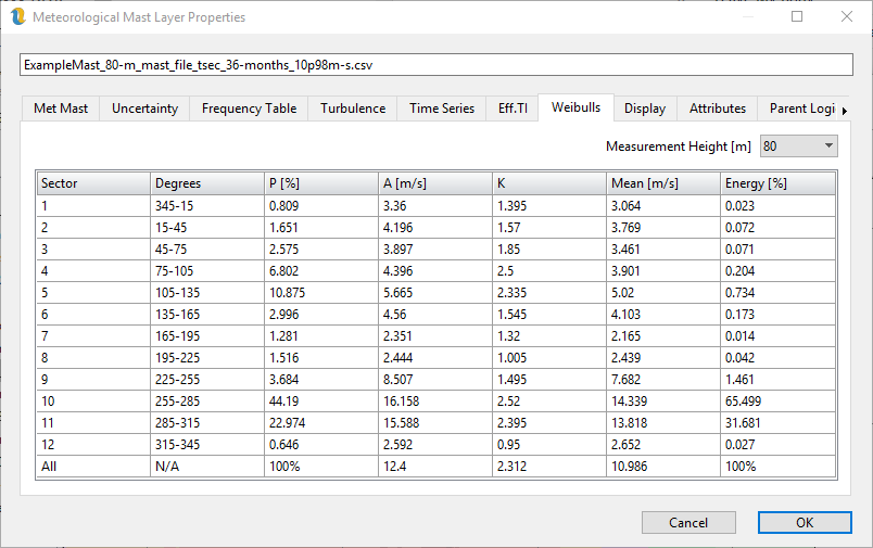
Figure 11: Met Mast Weibulls Tab