Energy-Losses
Users can assess and apply energy losses to both the standard frequency-based energy capture as well as the time-series energy capture routine. Openwind considers the gross energy to be the energy production before wake affects. However, this does not allow various control strategies (e.g. wind sector management, turbine scheduling, de-rating etc.) to be reported as losses. For this reason Openwind now has the notion of a theoretical gross which is the energy produced by simply combining the un-curtailed power curve with the un-waked wind speeds at the turbine location.
Time-series energy capture includes all the same losses as frequency table-based energy capture and so this section will describe the losses for the time-series energy capture but noting those losses which are only available in time-series mode.
Qualitatively the losses fall into two categories: modelled losses which are calculated for each calculation step; and percentage losses which are applied across all calculation steps.
All losses are reported as chained rather than as absolute fractions of the gross or wake-affected predicted energy yield. Because of this, in order to be able to convert between kWh losses and percentage losses, there needs to be a strict order and that is as follows:
| Loss | Modeled | Fixed % | Time-Series | Frequency-based |
|---|---|---|---|---|
| Markov Availability | x | x | ||
| High Temperature Shutdown | x | x | ||
| Low Temperature Shutdown | x | x | ||
| High Wind Hysteresis | x | x | ||
| Wind Sector Management | x | x | x | |
| Turbine Scheduling | x | x | ||
| Turbine De-rating | x | x | ||
| Array/Wake Effects | x | x | x | |
| Consumption | x | x | ||
| Icing | x | x | ||
| Additional Power Curve Loss | x | x | ||
| Under (sub-optimal) Performance | x | x | ||
| Turbulence Intensity* | x | x | x | |
| Inclined Flow | x | x | x | x |
| Icing | x | x | x | |
| Blade Soiling | x | x | x | |
| Blade Degradation | x | x | x | |
| Low Temperature Shutdown | x | x | x | |
| High Temperature Shutdown | x | x | x | |
| Site Access | x | x | x | |
| Lightning | x | x | x | |
| Other Environmental | x | x | x | |
| LACHWE (see below) | x | x | x | |
| Availability (contractual + non-contractual) | x | x | x | |
| Utility Grid Availability | x | x | x | |
| Grid Restart | x | x | x | |
| Substation Availability | x | x | x | |
| Power Curve Adjustment | x | x | x | |
| High Wind Hysteresis | x | x | x | |
| Wind Shear | x | x | x | |
| Sub-Optimal Performance | x | x | x | |
| Heating Package | x | x | x | |
| PPA Curtailment | x | x | x | |
| Environmental Curtailment | x | x | x | |
| Directional Curtailment | x | x | x | |
| Electrical | x | x | x | x |
| Grid Curtailment | x | x | ||
| “?” denotes a loss that could potentially be implemented at a future date. | ||||
| “*” denotes a loss that is marked for removal in a future update. |
Figure 1: Showing Order in Which Losses Are Applied
Some of the losses listed above are overt or potential duplications and in these cases it is up to the user to decide which to use. For instance, the transition matrix used to model time-series availability will ideally take account of all forms of availability loss and so can make several other availability loss categories redundant.
The losses are reported in the same order as in the table above in an attempt to facilitate the conversion to and from percentage and kWh losses.
As many of the modelled losses are defined as properties of the turbine type and therefore including in the [turbine type settings](Turbine Types), the following will focus predominantly on the fixed percentage losses.
Performance
Figure 2: Turbine Performance Tab
Turbine performance losses (figure 2) can be modelled as part of the turbine type or using the settings below:
Additional Power Curve Loss is provided to capture losses not described or modelled elsewhere. It can be run in TSEC mode as a power curve shift by checking the box to the right.
High Wind Control Hysteresis is best modelled in the turbine type in TSEC mode but can be input here as a simple chained loss.
Wind Shear can be specified as a simple loss here but again is probably best modelled in the PCA tab of the turbine type.
Sub-Optimal Performance is another performance loss which can be specified by the user and modelled as a power curve shift in TSEC by checking the box to the right.
Inclined Flow—this loss requires the Enterprise version of the software as well as access to inflow angle information. Inflow angles must be calculated by direction for every point in the site. Inflow angle information is available from CFD models or can be calculated as part of a wind map calculation. Inflow angle loss can alternatively be applied as a bulk loss.
Turbulence Loss (deprecated)—when checked, an energy loss is applied direction-by-direction, proportional to the total turbulence intensity at 15m/s (TI15). This option is being superseded by turbine manufacturers providing families of power curves by TI range. Also the PCA tab of the [turbine type settings](Turbine Types) makes this option redundant and it has been marked for removal from a future version.
Availability
Figure 3: Availability Losses Tab
Availability losses (figure 3) due to various factors - These are all user-inputs with the exception of the ability to calculate losses attributed to the correlation of downtime with high wind events (LACHWE) which, if selected, uses a proprietary UL method based on empirical data. The LACHWE loss can be either time or production based and is calculated differently depending on the choice the user makes.
Contractual and non-contractual have been separated out for reporting purposes. They are added together and chained as a single percentage loss but the contribution of each is noted in the energy capture report.
The option to model availability as a Markov chain is intended to allow the creation of a more realistic looking time-series output. Transition matrices can be pasted in directly or can be constructed in a separate interface accessed through pressing the Matrix Maker button. Users can specify different transition matrices by season using time-query objects. Use the Edit, Add and Delete buttons to manage multiple transition matrices.
The option to “Use single random number to switch states (recommended)” is a recent improvement and is the more correct way to run the Markov availability model. However, we have made it optional in order to allow for backwards compatibility. In previous versions two different random numbers were used and this mode is still available to use by unchecking this option.
All time-series energy captures start out as having all turbine operating normally (top-left of the transition matrix) and then for each time-step, pseudo-random numbers are generated and used to index into the transition matrix in order to determine if a change in availability has taken place. For the matrix show in figure 3 there is a 92% chance that the wind farm will stay in its current state. Should a state change take place, another random number is rolled to find out how many turbines were switched on or off. Although any box in the transition matrix can refer to multiple turbines, turbines are only switched on or off when moving between different cells in the transition matrix.
If the availability ever drops to zero, the plant restart lag time is activated and all turbines remain unavailable till the specified amount of time has passed.
Transition matrices are provided for summer and winter and represent reasonable defaults but are really only provided to allow users to experiment. In cases where a time-series is not available, Openwind provides a rudimentary capability to create reasonably realistic transition matrices.
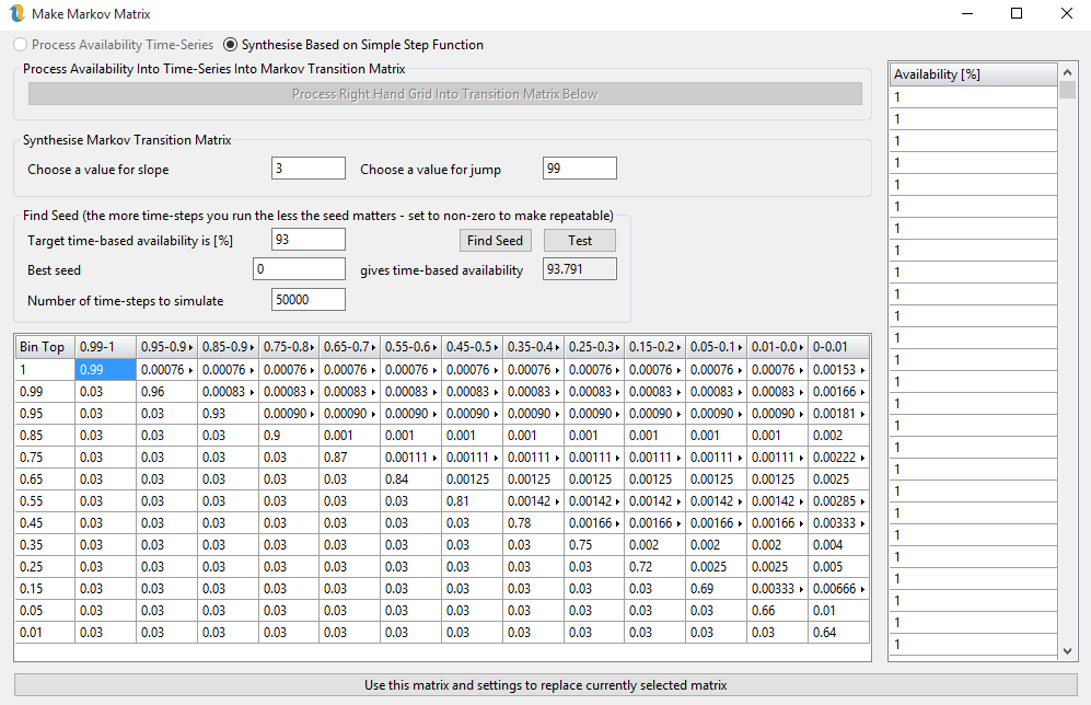
Figure 4: Matrix Maker Dialog Box
The option to process availability time-series enables the button that will process an availability time-series in the right-hand grid into a transition matrix. The availability time-series can be as fraction of turbines available or as the number of turbines. Openwind will auto-range in order to figure out what has been entered.
When processing a time-series in to Markov transition matrix, Openwind will ask you if you want to keep the default bin or specify a number of even spaced bins. The ideal, in terms of reproducing the original availability distribution in the time-series data, is to use the number of turbines plus 1 (for zero turbines). If you have a lot of turbines, you may want to divide that by an integer factor but still add an extra bin for all turbines being off. Once you have a lot of bins, the user-interface can get hard to read but this will not affect the functioning of the model.
This dialog can be used to play around with the influence of different seed variables although over sufficient records, the time-based availability becomes insensitive to seed value and so a non-zero seed will simply ensure that the time-series results are perfectly repeatable. Leaving the seed as zero will randomise the random number generator each time.
Openwind uses two parameters to create a new transition matrix. Slope refers to the number used on the bottom left half of the transition matrix to increment towards the leading diagonal. Higher values of the slope variable will translate into an easier recovery of the wind farm towards 100% available. Jump is the level to which cumulative availability jumps along the leading diagonal of the transition matrix. Changing either the jump or the slope will result in the immediate creation of a new transition matrix with those properties. If this was inadvertent, simply cancel out of this dialog using the cross in the top right of the dialog.
Pressing the test button will run the specified number of time-steps and update the box below to show the availability that was found. Setting the best seed to zero and repeatedly pressing the test button will give an idea of the range of results which might be expected. Setting the best seed to anything non-zero will yield the same results for a given transition matrix every time the test button is pressed. If the synthesise matrix options are enabled, then testing will fill the right-hand grid with the modelled time-series.
Electrical
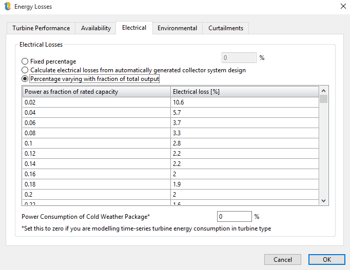
Figure 5: Electrical Losses Tab
Electrical losses (figure 5) can be a user-input fixed percentage or Openwind can calculate the electrical losses based on the collector system created by the cost of energy module. In order to use the electrical loss calculator, the workbook must be setup for cost of energy optimisation and all turbines must be reachable with the current electrical system settings. The electrical loss module assumes nominal voltages and will, therefore, tend to be slightly conservative in terms of line losses. At present it does not take account of power factor compensation. See Section below for information on setting up and using the electrical losses calculation.
Environment
Figure 6: Environmental Losses Tab
The Environmental energy losses (figure 6) can be defined in different ways depending on the loss. It is possible for the user to input a fixed value for any of the items on this page by checking the check box and inputting a value in percent. However, the default is for these losses to be spatially varying and determined by raster layers whose interpretation has been set to that particular loss type.
In addition to being able to calculate the losses from loss rasters, it is also possible to calculate the low/high temperature shutdown loss using the time series energy capture. If a time series energy capture is run with the option checked to “Include effects of low and high temperature shutdown” then this will override any value entered above or present in a raster.
The checkboxes on the right-hand side allow the blade soiling loss and the blade degradation loss to be run as power curve shifts in TSEC mode which are then iterated to give either the user-input or the raster-provided value depending on the states of the left hand check-boxes. In frequency domain energy capture they will both be run as simple chained efficiency losses.
Curtailments
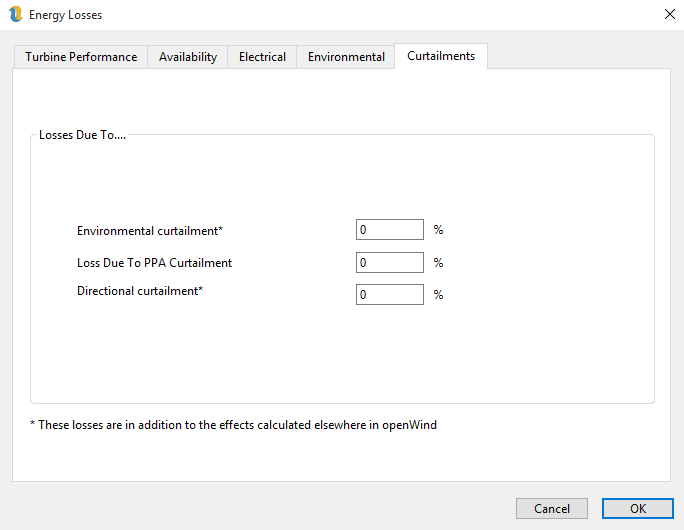
Figure 7: Curtailment Losses
The Curtailment losses tab (figure 7) specifies losses due to various curtailments. It is important to keep track of whether a curtailment is modelled elsewhere in the software and if so these curtailments should be set to zero or will be additional.