The following examples were originally submitted as part of a proposal to standardise the implementation of Annex E of Edition 4 of IEC61400-1. For the most part, the original wording and presentation has been preserved, but with the modifications described above. Our thanks and acknowledgements to the authors of this method. Given that we do not currently know who the authors were and that this was only shared as part of a discussion document and was not officially adopted as part of the standard, we preserve it here for posterity.
A series of examples are included below to show the selection of I start and the calculation of the turbine density. In the plots below turbines with a neighbour closer the <3 are shown as cyan circles, turbine without a close neighbour are shown with blue circles.
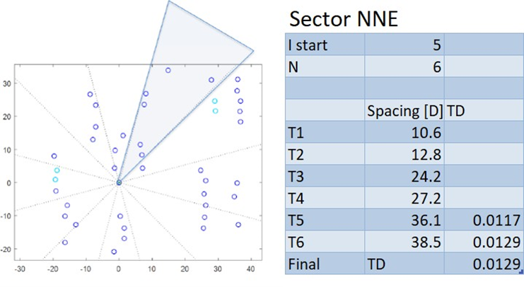
Figure A-1: Example of Turbine Density calculation for NNE sector of the example park
In the NNE sector there are no turbines spaced closer than 3D, so I start =5. The fifth turbine has a spacing of 36.1D, the 6th turbine of 38.5D. Filling in equation E.38.7 gives a turbine density of 0.0117 for the area up to T5, and 0.0129 for the area up to T6. The turbine density for that sector is the higher of these values namely 0.0129.
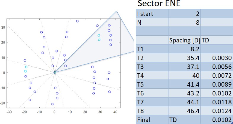
Figure A-2: Example of Turbine Density calculation for the ENE sector of the example park
In ENE sector of the park the second turbine has a neighbour closer than 3D, so I start is 2. The table shows the calculation of the turbine density for each of the neighbours. The highest turbine density is found using T8 and is 0.0124.
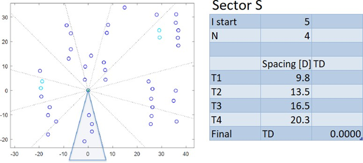
Figure A-3: Example of Turbine Density calculation for the ENE sector of the example park
In the southern sector there are only 4 neighbours, none of which has neighbours closer than 3D. So, then the number of turbines in the sector is less than istart. No wind farm added TI is applied in this sector.
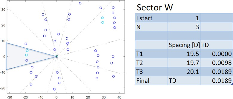
Figure A-4: Example of Turbine Density calculation for the ENE sector of the example park
In the eastern sector there are 3 turbines, two of which have neighbours closer than 3D, including the closest one, so istart = 1. The highest turbine density is found if all 3 turbines are considered, namely 0.028.
Examples and comparison with original proposal:
All examples below use a uniform wind rose, Ct from the IEA 10MW offshore test turbine and class B turbulence for the ambient TI including
Example 1. Big wind uniform wind farm with 4x5D spacing (dr*df=20).
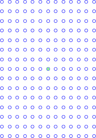
Figure A-5: Large Uniform Wind Park, with reference wind turbine marked with a green cross
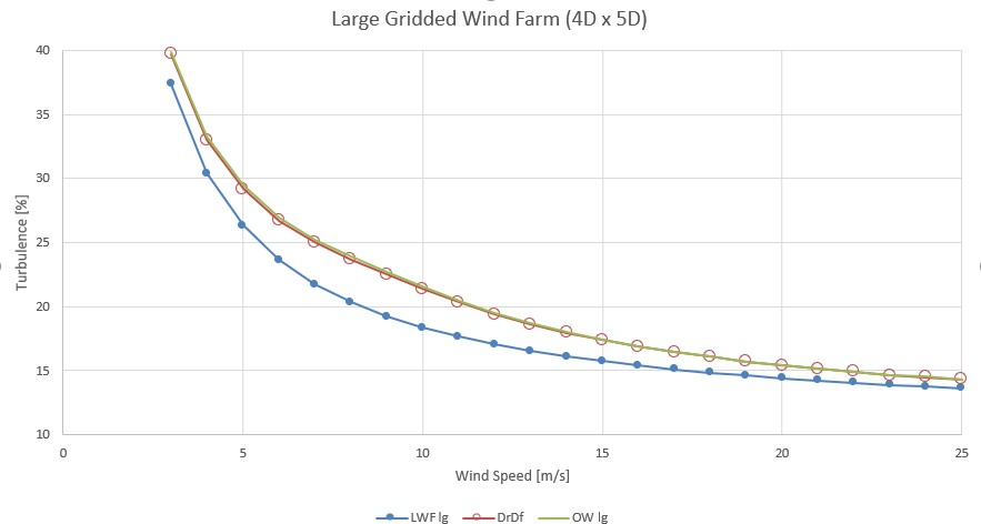
Figure A-6: Wind Farm Ambient TI for the Large Uniform Wind Park, from current and proposed method
Both methods result in the same ambient TI with windfarm effects
Example 2: Smaller, tightly spaced windfarm with 2.5x5D spacing (dr*df=12.5)
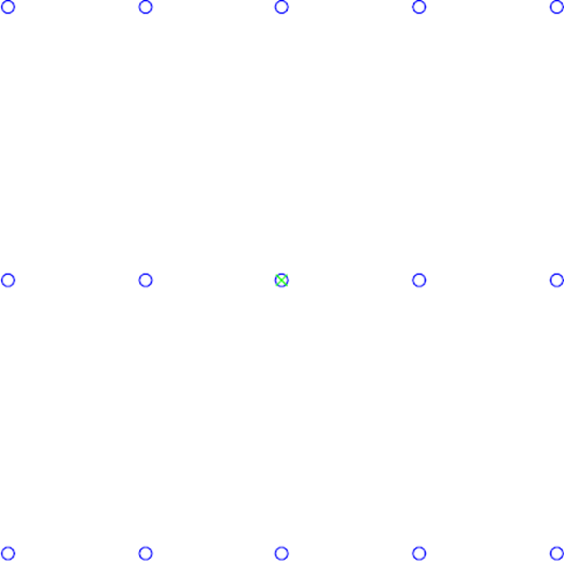
Figure A-7: Tightly Spaced Uniform Wind Park, with reference wind turbine marked with a green cross
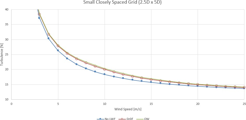
Figure A-8: Wind Farm Ambient TI for the Tightly Spaced Uniform Wind Park, from current and proposed method.

Figure A-9: Single row uniform wind park
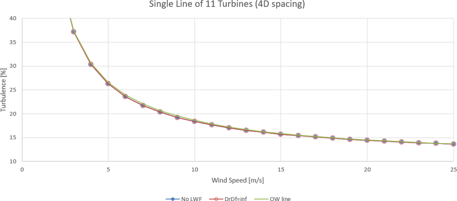
Figure A-10: Wind Farm Ambient TI for the Single row Uniform Wind Park, from current and proposed method.
With the use of i-1 instead of i in equation 38.7, the calculated LWF effect is very similar to that found using the much simpler Dr.Df in all the examples above. For this reason it has been adopted universally in Openwind whenever this effect is enabled.